实现属于自己的TensorFlow(三) - 反向传播与梯度下降实现
前言
上一篇介绍了损失函数对计算图中节点梯度计算的方法和实现以及反向传播算法的原理,但是并没有给出如何实现损失函数从后向前计算梯度。本文主要总结在可以计算每个节点梯度的基础上如何实现反向传播计算变量的梯度以及通过反向传播算法得到的梯度实现梯度下降算法优化来优化节点中的参数。最后我们使用实现的simpleflow完成一个线性回归模型的优化。
附上simpleflow代码: https://github.com/PytLab/simpleflow
正文
反向传播计算梯度的实现
再拿出上篇中用于解释反向传播算法的计算图:
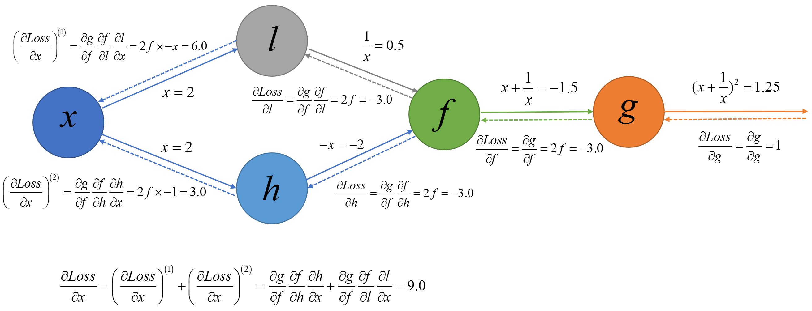
而且上篇中针对图中的每个节点中输出对输入的梯度计算进行了实现,现在我们实现需要从后向前反向搜索与损失节点相联系的节点进行反向传播计算梯度。通过上面我们知道若我们需要计算其他节点关于$g$的梯度我们需要以损失节点为起点对计算图进行广度优先搜索,在搜索的过程中我们使用上篇中实现的针对每个节点的梯度计算便可以一边遍历一边计算计算节点对遍历节点的梯度了。我们可以使用一个字典将节点与梯度进行保存。
这里需要注意的一点是,我们在上一篇针对每个节点计算梯度是损失值$Loss$对该节点输入的梯度,用公式表示就是针对一个$f$节点的操作$y = f(x, y)$, 我们计算的梯度为$\frac{\partial Loss}{\partial x}$和$\frac{\partial Loss}{\partial y}$, 如下图:
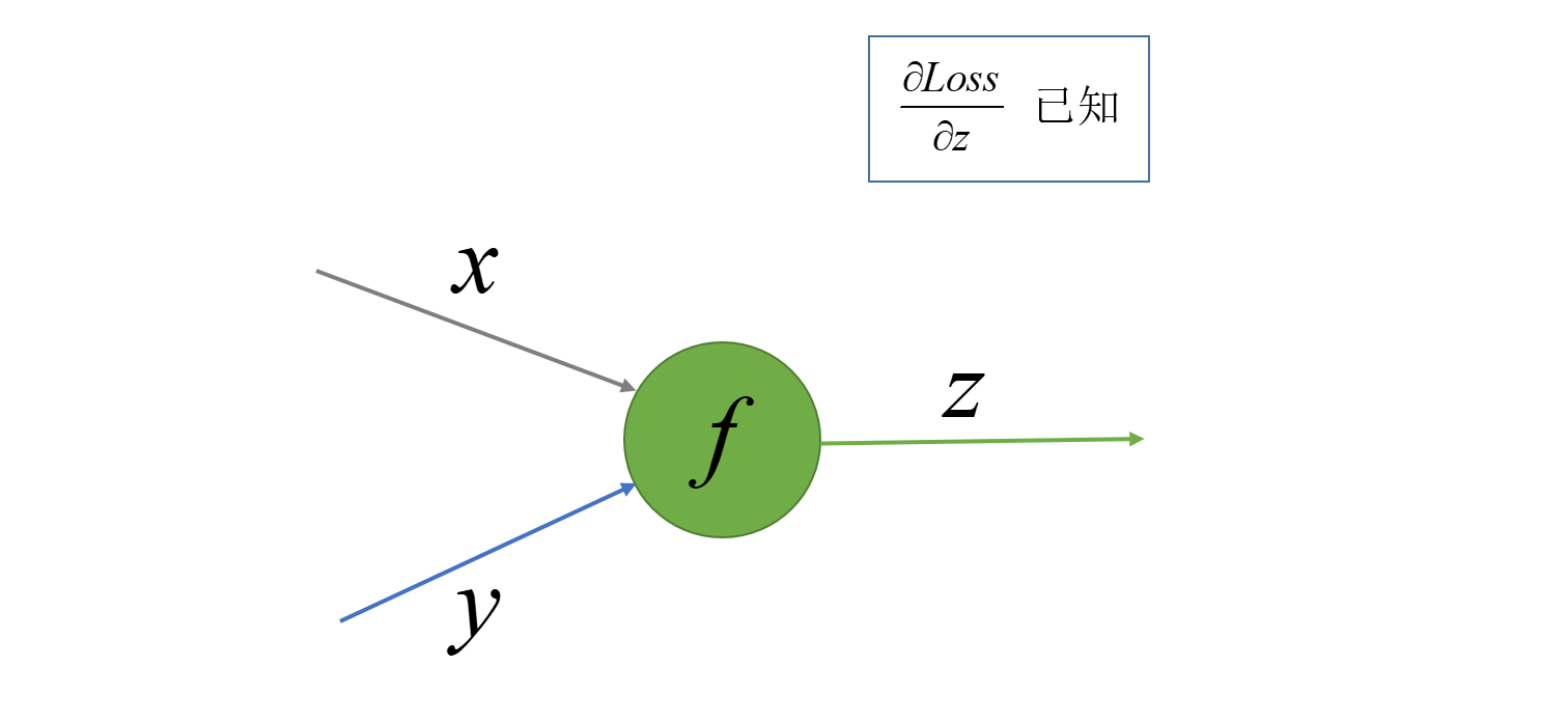
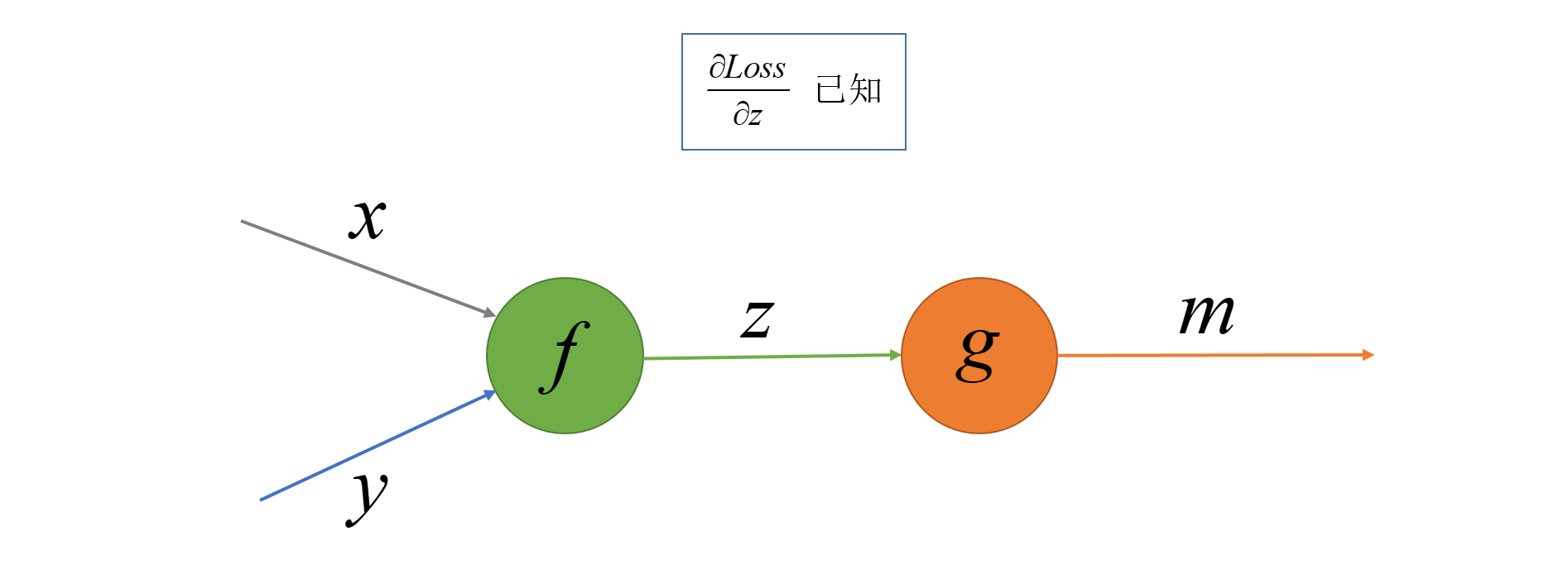
而在广度优先搜索的时候我们访问一个节点时候计算的梯度是损失值$Loss$对此节点的输出$z$的梯度, 也就是当我们遍历访问到节点$y = f(x, y)$的时候计算的梯度为$\frac{\partial Loss}{\partial f}$或者$\frac{\partial Loss}{\partial z}$, 其中$g$为操作节点的输出节点, 如下图. 若当前访问的节点有多个输出,我们就计算损失函数$Loss$对多个输出分别的梯度再求和。
区别了上面的梯度,我们就可以使用Python来实现计算图的广度优先搜索了, 广度优先搜索实现这里不多做赘述了, 就是使用一个先进先出(FIFO)队列控制遍历顺序,一个集合对象存储已访问的节点防止重复访问,然后遍历的时候计算梯度并将梯度放到grad_table中。广度优先搜索细节可以参考Breadth-first search
梯度计算实现如下(https://github.com/PytLab/simpleflow):
1 | def compute_gradients(target_op): |
梯度下降优化
梯度(最速下降)法
上面我们实现了损失函数对其他节点梯度的计算,得到梯度的目的是为了能够优化我们的参数,本部分我们实现一个梯度下降优化器来完成参数优化的目的。关于梯度下降优化的过程其实很简单,它基于以下的观察:
对于实值函数$F(x)$在$a$处可微且有定义,则函数$F(x)$在$a$点沿着梯度方向的反方向$-\nabla F(a)$下降最快。
梯度下降法就是以梯度的反方向作为每轮迭代的搜索方向然后根据设定的步长对局部最优值进行搜索。 而步长就是我们的学习率。
迭代公式
$$
x^{(k+1)} = x^{(k)} + \lambda_{k}d^{(k)}
$$
- 搜索方向: $d^{(k)} = -\nabla f(x^{(k)})$, 也称为最速下降方向
- 搜索步长: $\lambda_{k}$, 可以固定位某值也可以变化如指数衰减或者通过一维搜索取最优步长等
梯度算法步骤
- 取初始点$x^{(1)} \in \mathbb{R}^n$, 允许误差$\epsilon > 0$, 令$k = 1$;
- 计算搜索方向$d^{(k)} = -\nabla f(x^{(k)})$;
- 若$\lVert d^{(k)} \rVert \le \epsilon$, 则停止计算, $x^{(k)}$为所求极值点; 否则, 获取步长$\lambda_{k}$;
- 令$x^{(k+1)} = x^{(k) + \lambda_{k}d^{(k)}}$, 令$k:=k+1$转到第2步
对于一个二元函数$x^{(k)}$的移动轨迹类似下图:
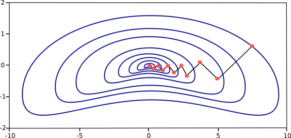
对于一个一元函数的局部极小值附近$x^{(k)}$的移动轨迹类似下图:
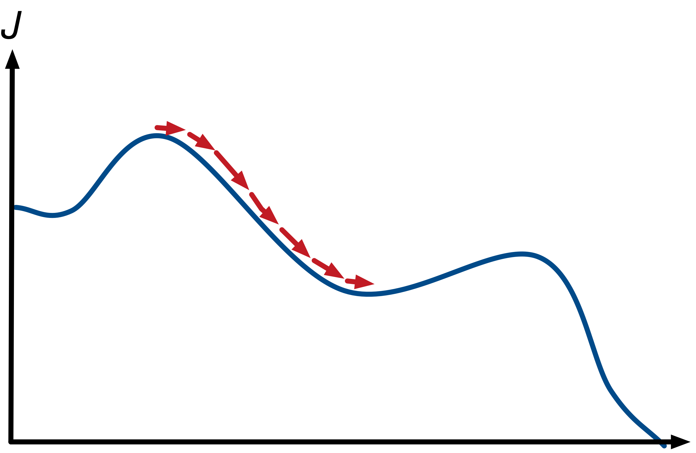
上面的流程中的终止条件是梯度收敛,在训练神经网络的时候我们需要根据自己的需要终止迭代,例如根据分类的准确度,均方误差或者迭代步数等.
使用梯度下降优化计算图中的参数
上面介绍了梯度下降算法通用的算法过程描述,这里将其应用在我们计算图中参数的优化。过程基本是一致的,只是我们现在的$x^{(k)}$变成了计算图中的参数(或者神经网络中的权重)值$W$了:
- 随机初始化变量$W$和$b$;
- 根据$W$和$b$计算损失函数值$Loss$, 若满足终止条件,则终止迭代
- 计算损失函数$Loss$对$W$和$b$的梯度值$G_W$, $G_b$;
- 沿着梯度反方向更新$W = W - rate \times G_W$和$b = b - rate \times G_b$;
- 返回到2
实现梯度下降优化器
好了,知道了算法的过程,我们需要给我们的simpleflow添加一个优化器,他的作用是根据当前图中节点的值计算图中所有可训练的trainable的变量节点中变量的梯度,并沿着梯度方向进行一步更新。
为了模仿tensorflow的接口,我们也定义一个GradientDescentOptimizer并在里面定义一个minimize方法来返回一个优化操作使其可以在session中执行, 代码如下:1
2
3
4
5
6
7
8
9
10
11
12
13
14
15
16
17
18
19
20
21
22
23
24
25
26
27
28
29
30
31
32
33class GradientDescentOptimizer(object):
''' Optimizer that implements the gradient descent algorithm.
'''
def __init__(self, learning_rate):
''' Construct a new gradient descent optimizer
:param learning_rate: learning rate of optimizier.
:type learning_rate: float
'''
self.learning_rate = learning_rate
def minimize(self, loss):
''' Generate an gradient descent optimization operation for loss.
:param loss: The loss operation to be optimized.
:type loss: Object of `Operation`
'''
learning_rate = self.learning_rate
class MinimizationOperation(Operation):
def compute_output(self):
# Get gradient table.
grad_table = compute_gradients(loss)
# Iterate all trainable variables in graph.
for var in DEFAULT_GRAPH.trainable_variables:
if var in grad_table:
grad = grad_table[var]
# Update its output value.
var.output_value -= learning_rate*grad
return MinimizationOperation()
使用simpleflow进行线性回归
综合前两篇以及本篇的内容,我们实现的计算图已经可以进行简单的模型训练了,本部分就以一个简单的线性模型为例子来看看成果。
生成数据
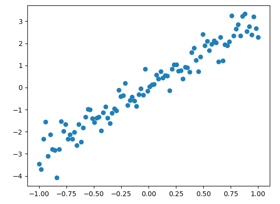
这里我们先基于$y=3x$生成加入一些噪声数据用于回归.1
2
3
4import numpy as np
input_x = np.linspace(-1, 1, 100)
input_y = input_x*3 + np.random.randn(input_x.shape[0])*0.5
构建计算图
下面我们来构建线性回归的计算图,线性回归的公式很简单而且只需要两个参数$w$和$b$,我们根据公式$y = wx + b$来构建计算图:
1 | import simpleflow as sf |
损失函数
这里我们使用平方差来作为损失函数:1
loss = sf.reduct_sum(sf.square(y - y_))
创建梯度下降优化器来训练模型
1 | train_op = sf.GradientDescentOptimizer(learning_rate=0.005).minimize(loss) |
输出:1
2
3
4
5
6
7
8
9
10
11
12
13
14
15
16
17
18
19
20
21step: 0, loss: 147.31229301332186, mse: 1.4731229301332187
step: 1, loss: 75.2862864776536, mse: 0.7528628647765361
step: 2, loss: 44.009064387253, mse: 0.44009064387253
step: 3, loss: 30.387486500361295, mse: 0.30387486500361294
step: 4, loss: 24.455137917985002, mse: 0.24455137917985004
step: 5, loss: 21.871534168474543, mse: 0.21871534168474543
step: 6, loss: 20.746346017138585, mse: 0.20746346017138584
step: 7, loss: 20.256314070038826, mse: 0.20256314070038825
step: 8, loss: 20.042899710055327, mse: 0.20042899710055326
step: 9, loss: 19.949955384044085, mse: 0.19949955384044085
step: 10, loss: 19.90947709692998, mse: 0.19909477096929978
step: 11, loss: 19.891848352949488, mse: 0.19891848352949487
step: 12, loss: 19.884170838991114, mse: 0.19884170838991114
step: 13, loss: 19.880827196321707, mse: 0.19880827196321707
step: 14, loss: 19.879371002772437, mse: 0.19879371002772436
step: 15, loss: 19.8787368142952, mse: 0.19878736814295198
step: 16, loss: 19.878460618163945, mse: 0.19878460618163946
step: 17, loss: 19.878340331678682, mse: 0.19878340331678682
step: 18, loss: 19.878287945577295, mse: 0.19878287945577294
step: 19, loss: 19.878265130847833, mse: 0.19878265130847833
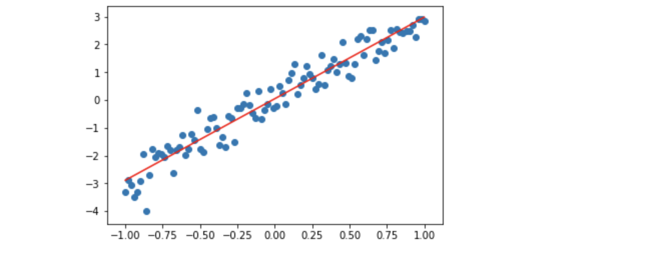
w: [[ 2.93373825]], b: 0.04568701269996128
绘制回归线
1 | w_value = float(w_value) |
总结
本文主要实现了计算图中的反向传播算法计算梯度以及梯度下降法优化参数,最后以一个线性模型为例子使用simpleflow构建的图来进行优化。后续将会在新增几个操作节点和梯度的实现来使用simpleflow构建一个多层感知机来解决简单的回归和分类问题。